Deep Learning and Approximate Bayesian Computation for Finite-Sites Model Inference
Apr – Jul 2024 · Columbia University, New York, USA · Supervisor: Dr. Simon Tavaré
- Simulation-based inference
- Deep learning
- Genomics
Research internship at the Herbert and Florence Irving Institute for Cancer Dynamics (Columbia University), supervised by Dr. Simon Tavaré.
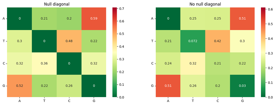
Understanding how DNA molecules evolve and mutate — over population time scales as well as within the human lifespan — is of major scientific interest. This project focused on DNA molecules suspected to have biased transition parameters (some nucleotide substitutions being favoured over others), which must be studied with a finite-sites approach. Their behaviour is described by multi-parametric stochastic evolutionary models that take a vector of parameters as input and output nucleotide sequences sampled from a population of individuals or cells.
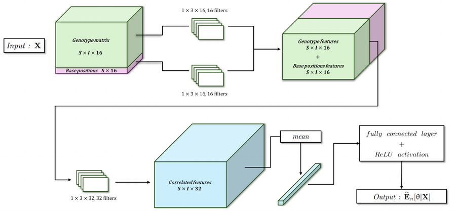
- Learning summary statistics. Complex, high-dimensional genomic data are compressed into a low-dimensional vector of summary statistics by a deep network inspired by Sanchez et al. (2021), which I adapted to nucleotide sequences distinguishing the A, T, C and G bases.
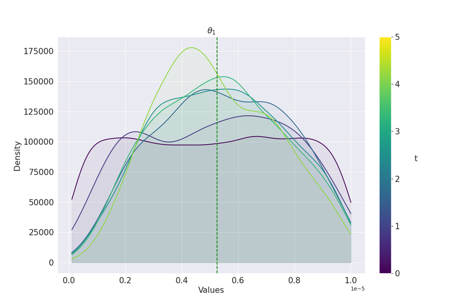
- Inference. The parameters of the stochastic model are then fitted to the observed data with an adaptive sequential Monte Carlo algorithm in which each step runs a random-forest Approximate Bayesian Computation (ABC-RF) on simulated data, yielding an increasingly precise posterior distribution.
The results show that the method can infer the parameters of a finite-sites model generating sequences with multiple non-visible mutations.